Lecture 18: Algorithmic Analysis
- Motivation
- Standard Approach
- Examples
- Simplifying with Worst Case and Big-O
- Recursive Examples
- Faster Euclidean
Motivation
Want to compare algorithms– particularly ones that can solve arbitrarily large instances.
We would like to be able to talk about the resources (running time, memory, energy consumption) required by a program/algorithm as a function f (n) of some parameter n (e.g. the size) of its input.
Example
How long does a given sorting algorithm take to run on a list of n elements?
Issues
Problems
- The exact resources required for an algorithm are difficult to pin down. Heavily dependent on:
- Environment the program is run in (hardware, software, choice of language, external factors, etc)
- Choice of inputs used
- Cost functions can be complex, e.g.
Need to identify the “important” aspects of the function.
Order of growth
Consider two time-cost functions:
- $f_1(n)=\frac{1}{10}n^2$ milliseconds, and
- $f_2(n)=10n log n$ milliseconds
| Input size | f1(n) | f2(n) |
|---|---|---|
| 100 | 0.01s | 2s |
| 1000 | 1s | 30s |
| 10000 | 1m40s | 6m40s |
| 100000 | 2h47m | 1h23m |
| 1000000 | 11d14h | 16h40m |
| 10000000 | 3y3m | 8d2h |
Standard Approach
Algorithmic analysis
Asymptotic analysis is about how costs scale as the input increases.
Standard (default) approach:
- Consider asymptotic growth of cost functions
- Consider worst-case (highest cost) inputs
- Consider running time cost: number of elementary operations
Take Notice
Other common analyses include:
- Average-case analysis
- Space (memory) cost
Elementary operations
Informally: A single computational “step”; something that takes a constant number of computation cycles.
Examples:
- Arithmetic operations
- Comparison of two values
- Assignment of a value to a variable
- Accessing an element of an array
- Calling a function
- Returning a value
- Printing a single character
Take Notice
Count operations up to a constant factor, O(1), rather than an exact number.
Examples
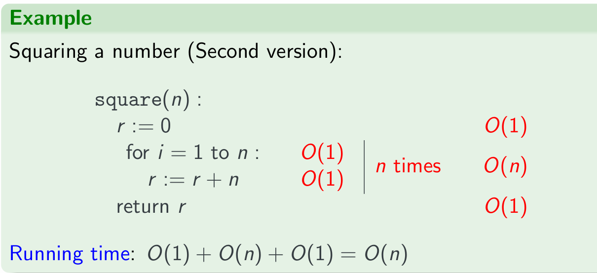
Squaring a number (First version):
square(n) :
    return n ∗ n // ------ O(1)
Running time: O(1)
Running time vs Execution time
Previous example shows one difference between running time and execution time.
In general, running time only approximates execution time:
- Simplifying assumptions about elementary operations
- Hidden constants in big-O
- Big-O only looks at limiting performance as n gets large.
Implementations of square(n) will take longer as n gets bigger
Squaring
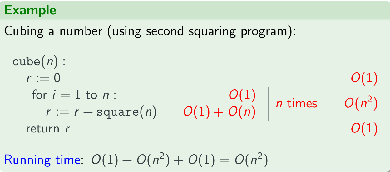
Cubing
Note the function square() is from the above algorithm, hence it’s n loop of $O(n) -> O(n^2)$
Simplifying with Worst Case and Big-O
Worst-case and big-O
Worst-case input assumption and big-O combine to simplify the analysis:
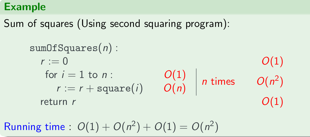
注意,这里的 for i = 1 to n: 这里的$O(1)$ 是 i=1,这里是 n times 所以整个for循环后面需要再 n times 成 $O(n^2)$。有循环的情况下,需要一层一层分析,先不考虑循环去看每个单独的执行语句进行和操作,再用for循环进行乘操作。
sum of Square
Take Notice
Simplifications might lead to sub-optimal bounds, may have to do a better analysis to get best bounds:
- Finer-grained upper bound analysis
- Analyse specific cases to find a matching lower bound (big-Ω)
Take Notice
Big-Ω is a lower bound analysis of the worst-case; NOT a “best-case” analysis.
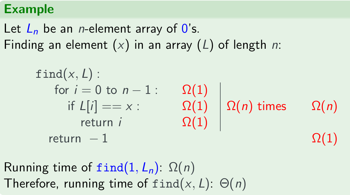
Analyse specific cases to find a matching lower bound (big-Ω)
Find an element from an array
Recursive Examples
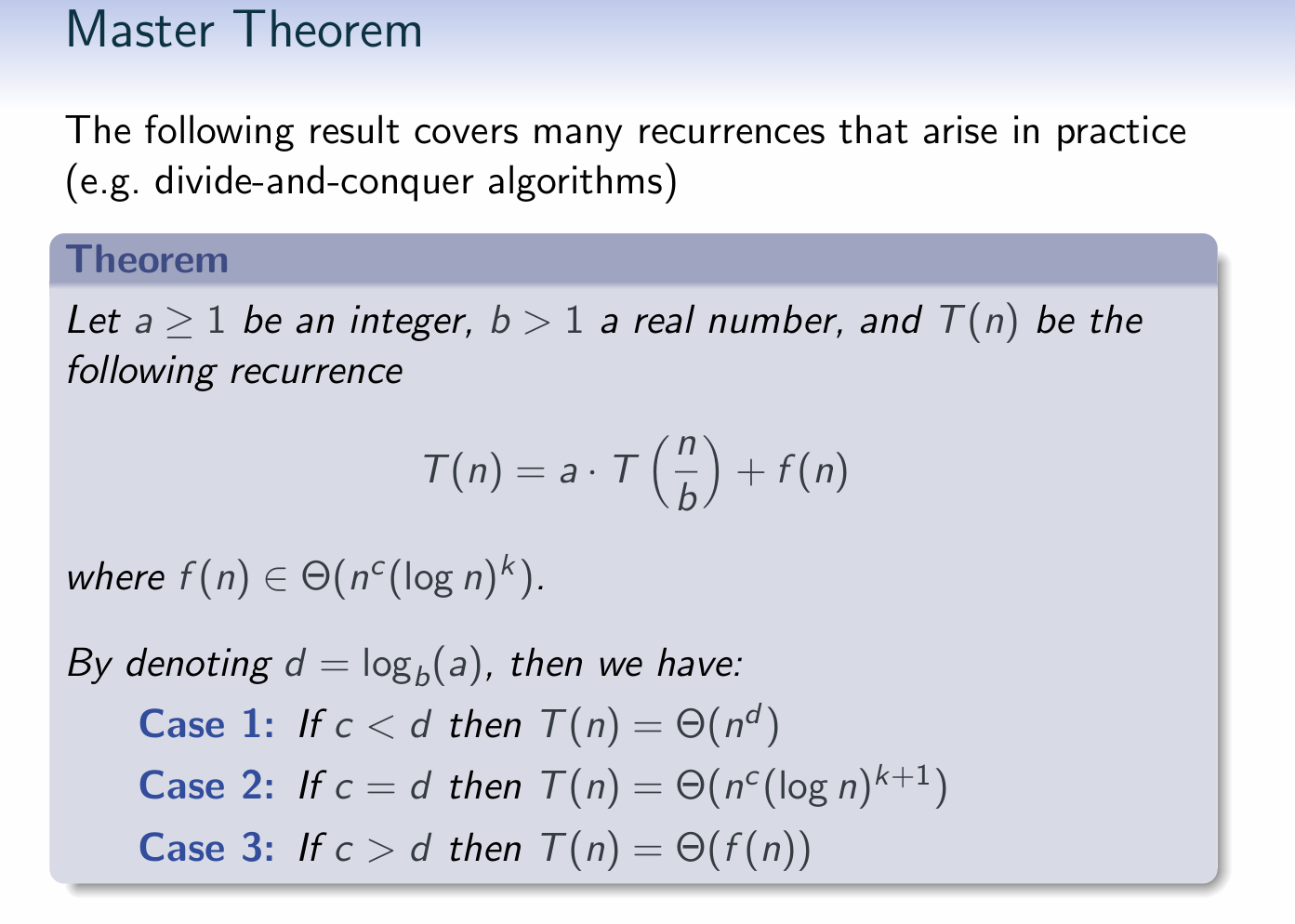
此处涉及了递归那里的“master theorem”
Factorial
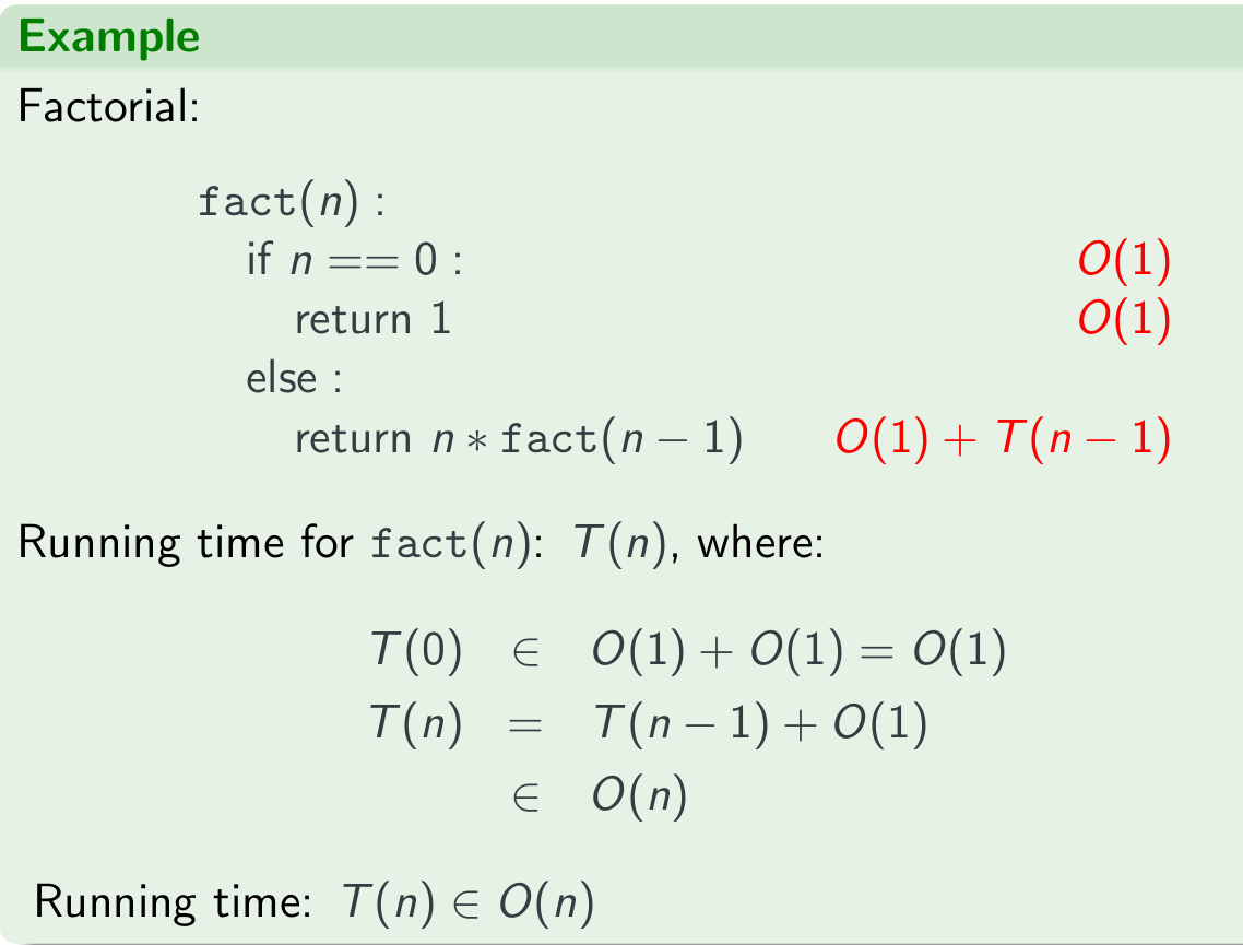
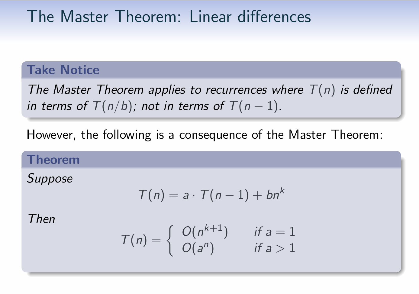
I listed the Master Theorem and Linear differences here, please regard the a=1 condition to apply the T(n) above.
Master Theorom
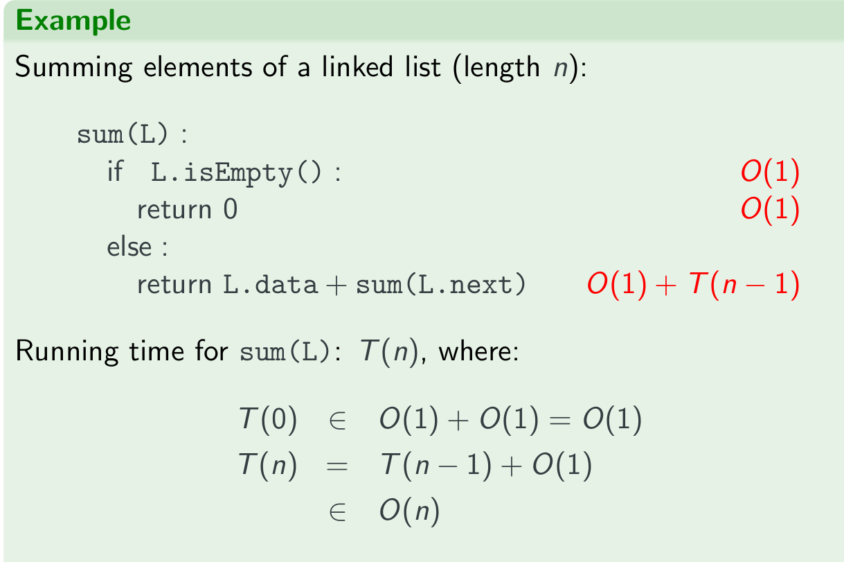
Sum elements of a linked list
the k=1, so it’s $O(n^{1+1})=O(n^2)$
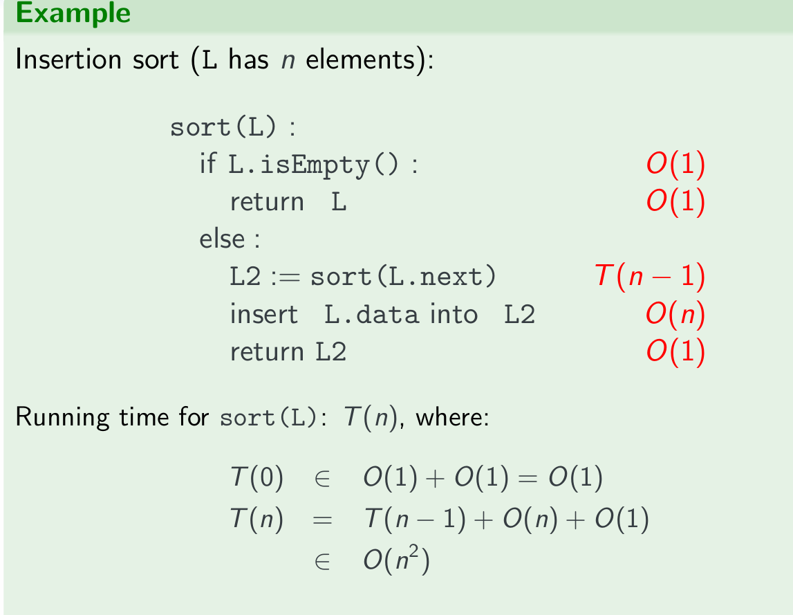
Insertion sort
Euclidean algorithm
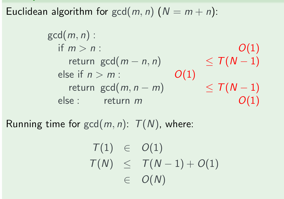
Recursive examples
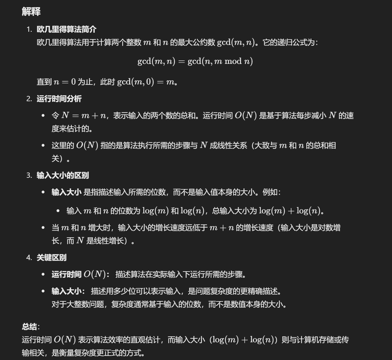
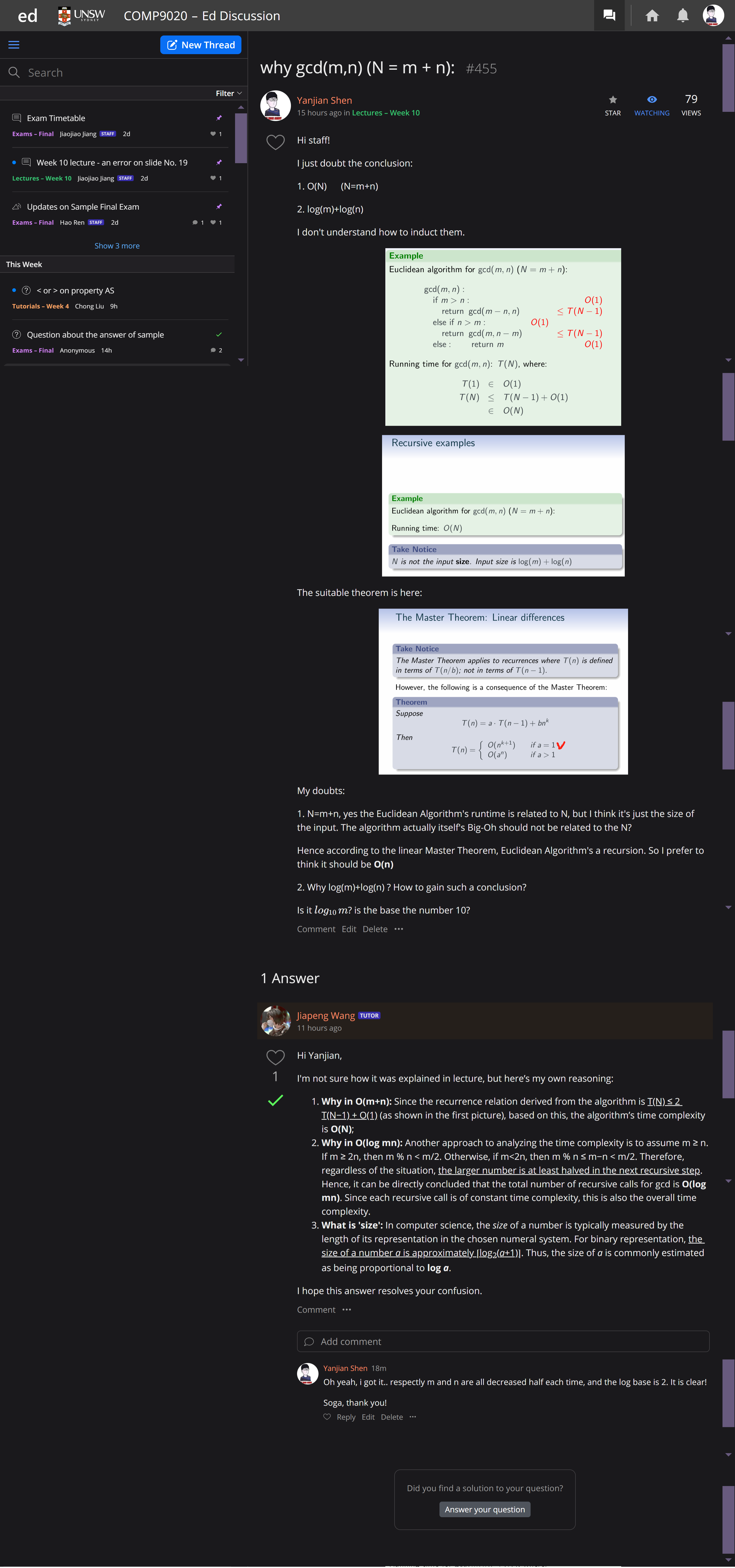
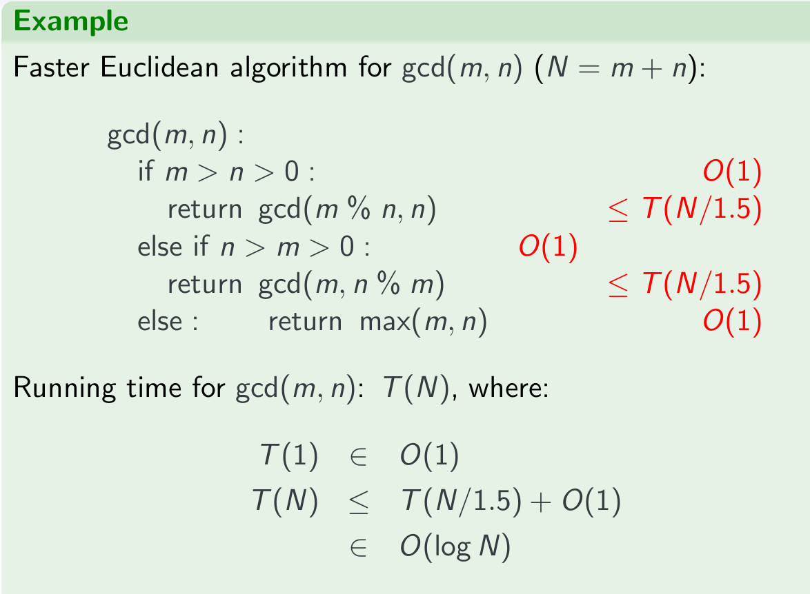
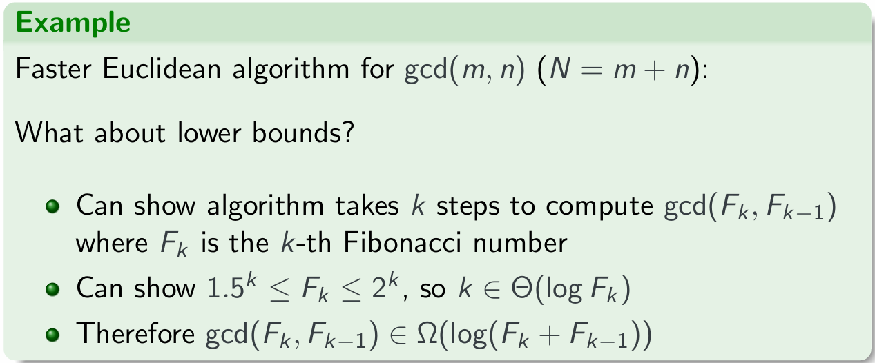
Euclidean algorithm for $gcd(m,n) (N = m + n)$:
Running time: $O(N)$
Take Notice
N is not the input size. Input size is $log(m) + log(n)$
Faster Euclidean
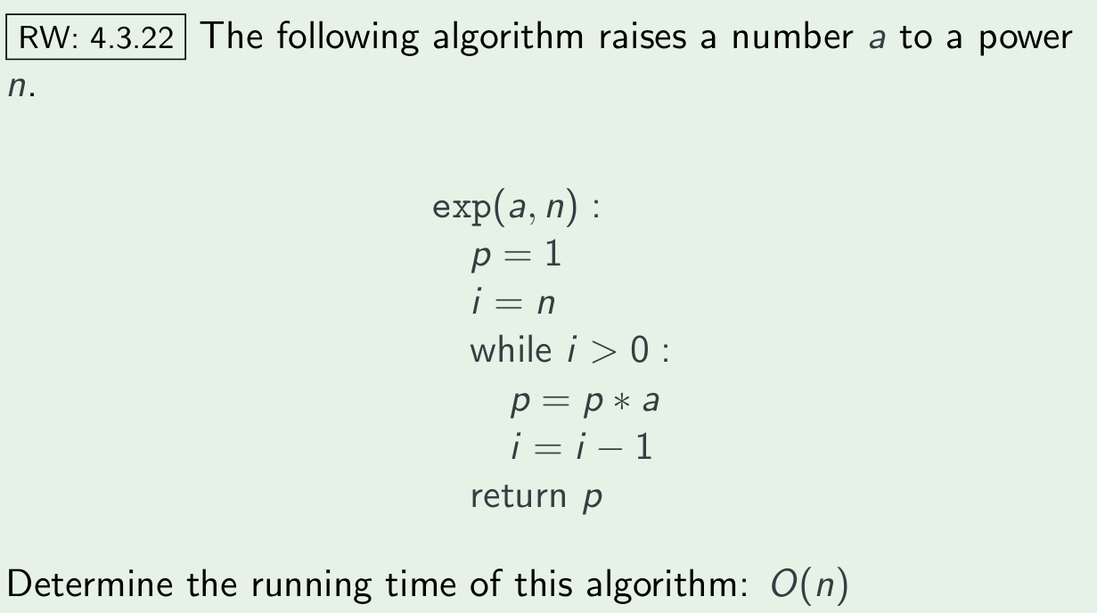
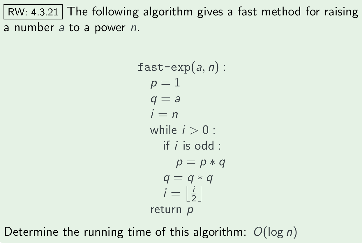
pow
Welcome to point out the mistakes and faults!