- NumPy文档
- 数组创建
- Array Indexing
- Datatypes
- Array Math
- transpose
- Broadcasting
- Matplotlib
- PyTorch Tensors
- Google colab
NumPy文档
https://numpy.org/doc/stable/user/basics.creation.html#arrays-creation
数组创建
1. a = np.zeros((2,2))
作用:创建一个 2×2 的全 0 数组
输出示例:
python
CopyEdit
[[0. 0.]
[0. 0.]]
2. b = np.ones((1,2))
作用:创建一个 1×2 的全 1 数组
输出示例:
python
CopyEdit
[[1. 1.]]
3. c = np.full((2,2), 7)
作用:创建一个 2×2 的数组,每个元素都是 7
输出示例:
python
CopyEdit
[[7 7]
[7 7]]
4. d = np.eye(2)
作用:创建一个 2×2 的单位矩阵(对角线为 1,其它为 0)
输出示例:
python
CopyEdit
[[1. 0.]
[0. 1.]]
5. e = np.random.random((2,2))
作用:创建一个 2×2 的数组,每个元素是 0~1 的随机小数
输出示例(每次运行结果不同):
python
CopyEdit
[[0.91 0.08]
[0.68 0.87]]
总结
这些是 numpy
中常用的数组初始化方法,非常适合用来创建矩阵、测试数据、或用于科学计算:
函数 说明
np.zeros 创建全 0 数组
np.ones 创建全 1 数组
np.full 创建指定值的数组
np.eye 创建单位矩阵
np.random.random 创建随机数组
Array Indexing
切片索引
a = np.array([
[1,2,3,4],
[5,6,7,8],
[9,10,11,12]
])\
b = a[:2, 1:3]
会输出
[[2 3]
[6 7]]
a[: 2, 1:3]
括号里,: 是行列操作的分隔符,冒号之前是 行 操作, 冒号之后是 列
操作
a = np.array([[1,2,3,4], [5,6,7,8], [9,10,11,12]])\
\
# Two ways of accessing the data in the middle row of the array.\
# Mixing integer indexing with slices yields an array of lower\
# rank, while using only slices yields an array of the same rank\
# as the original array:\
row_r1 = a[1, :] # Rank 1 view of the second row of a\
row_r2 = a[1:2, :] # Rank 2 view of the second row of a\
print(row_r1, row_r1.shape) # Prints \”[5 6 7 8] (4,)\”\
print(row_r2, row_r2.shape) # Prints \”[[5 6 7 8]] (1, 4)\”
[注意]{.mark}:切片以列表之姿出现:
a[1, :]
是说访问第1个元素(从0计起,1是第2行)(非切片),故而输出
[5 6 7 8] (4,)
a[1:2, :] 是说第1行元素(切片),故而输出
[[5 6 7 8]] (1, 4)
数组内数组选取
import numpy as np\
\
# Create a new array from which we will select elements\
a = np.array([[1,2,3], [4,5,6], [7,8,9], [10, 11, 12]])\
\
print(a) # prints \”array([[ 1, 2, 3],\
# [ 4, 5, 6],\
# [ 7, 8, 9],\
# [10, 11, 12]])\”\
\
# Create an array of indices\
b = np.array([0, 2, 0, 1])
arange
x = np.arange(-10, 10)
💡 解释:
-10 是起始值(包含)
10 是终止值(不包含)
默认步长是 1
所以这行代码会生成一个从 -10 到 9 的整数数组:
# Select one element from each row of a using the indices in b\
print(a[np.arange(4), b]) # Prints \”[ 1 6 7 11]\”\
\
# Mutate one element from each row of a using the indices in b\
# np.arange(4) 生成 [0, 1, 2, 3]:对应 4 行的行索引\
# b = [0, 2, 0, 1]:每一行中要选择的列索引\
# [相当于选取]{.mark}\
# [\
# a[0, 0], # 1\
# a[1, 2], # 6\
# a[2, 0], # 7\
# a[3, 1] # 11\
# ]
a[np.arange(4), b] += 10\
print(a) # prints \”array([[11, 2, 3],\
# [ 4, 5, 16],\
# [17, 8, 9],\
# [10, 21, 12]])
布尔索引操作
import numpy as np\
\
a = np.array([[1,2], [3, 4], [5, 6]])\
\
# 括号是可选的,不加括号也行\
[bool_idx = (a > 2)]{.mark} # Find the elements of a that are bigger
than 2;\
# this returns a numpy array of Booleans of the\
# same shape as a, where each slot of bool_idx\
# tells whether that element of a is > 2.\
\
print(bool_idx) # Prints \”[[False False]\
# [ True True]\
# [ True True]]\”
# We use boolean array indexing to construct a rank 1 array\
# consisting of the elements of a corresponding to the\
# True values of bool_idx\
print(a[bool_idx]) # Prints \”[3 4 5 6]\”\
[# 1. 在 bool_idx 为 True 的位置,取出对应的 a 中的元素。\
# 2. 将结果变成一个一维数组返回。]{.mark}
# We can do all of the above in a single concise statement:\
print(a[a > 2]) # Prints \”[3 4 5 6]\”
总结,
a是np数组,a>2本身已经是一个bool列表了,然后用作索引可以直接过滤出符合布尔的元素。
Datatypes
默认就是 int64 和 float64
import numpy as np
x = np.array([1, 2]) # Let numpy choose the datatype
print(x.dtype) # Prints \”[int64]{.mark}\”
x = np.array([1.0, 2.0]) # Let numpy choose the datatype
print(x.dtype) # Prints \”[float64]{.mark}\”
x = np.array([1, 2], dtype=np.int64) # Force a particular datatype
print(x.dtype) # Prints \”[int64]{.mark}\”
Array Math
import numpy as np\
\
x = np.array([[1,2],[3,4]], dtype=np.float64)\
y = np.array([[5,6],[7,8]], dtype=np.float64)
加
# Elementwise sum; both produce the array\
# [[ 6.0 8.0]\
# [10.0 12.0]]\
print(x + y)\
print(np.add(x, y))
减
# Elementwise difference; both produce the array\
# [[-4.0 -4.0]\
# [-4.0 -4.0]]\
print(x - y)\
print(np.subtract(x, y))
乘
*是逐个元素相乘,不是矩阵乘法
# Elementwise product; both produce the array\
# [[ 5.0 12.0]\
# [21.0 32.0]]\
print(x * y)\
print(np.multiply(x, y))
除
# Elementwise division; both produce the array\
# [[ 0.2 0.33333333]\
# [ 0.42857143 0.5 ]]\
print(x / y)\
print(np.divide(x, y))
开方
# Elementwise square root; produces the array\
# [[ 1. 1.41421356]\
# [ 1.73205081 2. ]]\
print(np.sqrt(x))
点乘(向量内积)
Note that * is elementwise multiplication, not matrix multiplication.
We instead use the dot function to compute inner products of vectors, to
multiply a vector by a matrix, and to multiply matrices. dot is
available both as a function in the numpy module and as an instance
method of array objects:
dot 在 NumPy 中,其行为取决于输入数组的维度:
两个向量(一维数组):执行点乘(inner product)。
矩阵和向量:执行矩阵乘向量。
两个矩阵:执行矩阵乘法。
如果要明确进行矩阵乘法,也可以使用 @ 作为运算符:
print(x @ v) # 等价于 x.dot(v)
print(x @ y) # 等价于 x.dot(y)
import numpy as np
x = np.array([[1,2],[3,4]])
y = np.array([[5,6],[7,8]])
v = np.array([9,10])
w = np.array([11, 12])
# Inner product of vectors; both produce 219
print(v.dot(w))
print(np.dot(v, w))
# Matrix / vector product; both produce the rank 1 array [29 67]
print(x.dot(v))
print(np.dot(x, v))
# Matrix / matrix product; both produce the rank 2 array
# [[19 22]
# [43 50]]
print(x.dot(y))
print(np.dot(x, y))
一维向量与一维向量的内积与外积
两个一维向量进行 dot(点乘)
a = np.array([1, 2, 3])
b = np.array([4, 5, 6])
print(a @ b) # 输出 32,相当于 1*4 + 2*5 + 3*6
print(np.dot(a, b)) # 也输出 32
这两个是点乘(scalar),不是矩阵乘。
想进行矩阵乘法,要明确转换维度
外积(Outer Product)
a_col = a.reshape(-1, 1) # shape: (3, 1)
b_row = b.reshape(1, -1) # shape: (1, 3)
print(a_col @ b_row)
[[ 4 5 6]
[ 8 10 12]
[12 15 18]]
这个就是一个 (3×1) × (1×3) 的矩阵乘法,结果是 (3×3) 的外积矩阵。
内积(行向量 × 列向量 → 标量)
a_row = a.reshape(1, -1) # shape: (1, 3)
b_col = b.reshape(-1, 1) # shape: (3, 1)
print(a_row @ b_col) # 输出 [[32]]
这是矩阵乘法 (1×3) @ (3×1),结果是 (1×1)。
transpose
# You can find the full list of mathematical functions provided by
numpy in the documentation.\
# Apart from computing mathematical functions using arrays, we
frequently need to reshape or otherwise manipulate data in arrays. The
simplest example of this type of operation is transposing a matrix; to
transpose a matrix, simply use the T attribute of an array object:\
\
# import numpy as np\
#\
# x = np.array([[1,2], [3,4]])\
# print(x) # Prints \”[[1 2]\
# # [3 4]]\”\
# # [T]{.mark}只是转置的临时视图,非永久更改\
# print(x.T) # Prints \”[[1 3]\
# # [2 4]]\”\
#\
# # Note that taking the transpose of a rank 1 array does nothing:\
# v = np.array([1,2,3])\
# print(v) # Prints \”[1 2 3]\”\
# print(v.T) # Prints \”[1 2 3]\”\
#\
# # 永久转置\
# a = np.array([[1, 2], [3, 4]])\
# [a = a.T # 现在 a 是转置后的版本]{.mark}\
# # 因为 .T
是个视图(共享内存),你如果之后还想避免原数组被影响,建议配合
.copy():\
# [a = a.T.copy()]{.mark}
Broadcasting
关于rank 秩
注意矩阵的 rank,翻译为 秩,可以理解为 一维向量 是矢量吗?不,得升级成和
矩阵 一样的维度、大小
Broadcasting is a powerful mechanism that allows numpy to work with
arrays of different shapes when performing arithmetic operations.
Frequently we have a smaller array and a larger array, and we want to
use the smaller array multiple times to perform some operation on the
larger array.
For example, suppose that we want to add a constant vector to each row
of a matrix. We could do it like this:
import numpy as np
# We will add the vector v to each row of the matrix x,
# storing the result in the matrix y
x = np.array([[1,2,3], [4,5,6], [7,8,9], [10, 11, 12]])
v = np.array([1, 0, 1])
[y = np.empty_like(x) # Create empty matrix with same shape as
x]{.mark}
# Add vector v to each row of matrix x with an explicit loop
[for i in range(4):]{.mark}
[y[i, :] = x[i, :] + v]{.mark}
# Now y is the following
# [[ 2 2 4]
# [ 5 5 7]
# [ 8 8 10]
# [11 11 13]]
print(y)
py的逐行相加(不推荐、慢)
-------------------- Broadcasting\
# import numpy as np\
#\
# # We will add the vector v to each row of the matrix x,\
# # storing the result in the matrix y\
# x = np.array([[1,2,3], [4,5,6], [7,8,9], [10, 11, 12]])\
# v = np.array([1, 0, 1])\
# y = np.empty_like(x) # Create empty matrix with same shape as x\
#\
# # Add vector v to each row of matrix x with an explicit loop\
# for i in range(4):\
# y[i, :] = x[i, :] + v\
#\
# # Now y is the following\
# # [[ 2 2 4]\
# # [ 5 5 7]\
# # [ 8 8 10]\
# # [11 11 13]]\
# print(y)
扩张较小rank再矩阵相加(也不推荐,因为并非最优写法)
-------------------- Broadcasting 2\
# This works; however when the matrix x is very large, computing an
explicit loop in Python could be slow. Note that adding the vector v to
each row of the matrix x is equivalent to forming a matrix vv by
stacking multiple copies of v vertically, then performing elementwise
summation of x and vv. We could implement this approach like this:\
\
# import numpy as np\
#\
# # We will add the vector v to each row of the matrix x,\
# # storing the result in the matrix y\
# x = np.array([[1,2,3], [4,5,6], [7,8,9], [10, 11, 12]])\
# v = np.array([1,0,1])\
# vv = np.tile(v,(4,1)) # Stack 4 copies of v on top of each other\
# print(vv) # Prints \”[[1 0 1]\
# # [1 0 1]\
# # [1 0 1]\
# # [1 0 1]]\”\
# y = x + vv # Add x and vv elementwise\
# print(y) # Prints \”[[ 2 2 4\
# # [ 5 5 7]\
# # [ 8 8 10]\
# # [11 11 13]]\”
使用np自带的广播相加
举例说明 + 详细解读
假设:
python
CopyEdit
import numpy as np
x = np.array([[1, 2, 3],
[4, 5, 6],
[7, 8, 9],
[10,11,12]]) # shape = (4, 3)
v = np.array([1, 0, 1]) # shape = (3,)
现在执行:
python
CopyEdit
y = x + v
步骤一:对齐维度数
x 的形状是 (4, 3),rank = 2
v 的形状是 (3,),rank = 1
根据规则1,要让维度数相同,在 v 形状前面补 1:
lua
CopyEdit
v.shape: (3,) --> (1, 3)
步骤二:判断各维度兼容性
维度 x v 是否兼容?
尺寸 尺寸
0 4 1 是(v在该维度为1,可以广播扩展)
1 3 3 是(尺寸相同)
两者在所有维度兼容,可以广播。
步骤三:计算广播后形状
广播后形状是两个数组形状在每维的最大值:
scss
CopyEdit
(4, 3) 和 (1, 3) --> (4, 3)
步骤四:扩展数组(虚拟复制)
x 保持 (4, 3) 形状不变。
v 沿着第0维”复制”4次,变成:
lua
CopyEdit
[[1, 0, 1],
[1, 0, 1],
[1, 0, 1],
[1, 0, 1]]
步骤五:逐元素相加
lua
CopyEdit
[[ 1+1, 2+0, 3+1],
[ 4+1, 5+0, 6+1],
[ 7+1, 8+0, 9+1],
[10+1, 11+0, 12+1]]
=>
[[ 2, 2, 4],
[ 5, 5, 7],
[ 8, 8, 10],
[11, 11, 13]]
3. 额外举例 —- 维度更复杂
假设:
python
CopyEdit
a = np.ones((3, 4, 5)) # shape (3,4,5)
b = np.ones(( 4, 1)) # shape (4,1)
补维度,b 形状补成 (1,4,1)
逐维比较:
维度 a 尺寸 b 尺寸 兼容?
0 3 1 是,b沿该维度广播扩展3次
1 4 4 是,尺寸相同
2 5 1 是,b沿该维度广播扩展5次
广播形状为 (3, 4, 5)
代码示例
-------------------- Broadcasting 3\
import numpy as np\
\
# We will add the vector v to each row of the matrix x,\
# storing the result in the matrix y\
x = np.array([[1,2,3], [4,5,6], [7,8,9], [10, 11, 12]])\
v = np.array([1, 0, 1])\
y = x + v # Add v to each row of x using broadcasting\
print(y) # Prints \”[[ 2 2 4]\
# [ 5 5 7]\
# [ 8 8 10]\
# [11 11 13]]\”
# Another solution is to reshape w to be a column vector
# of shape (2, 1); we can then broadcast it directly
# against x to produce the same output.
print(x + np.reshape(w, (2, 1)))
# Multiply a matrix by a constant: x has shape (2, 3).
# Numpy treats scalars as arrays of shape ();
# these can be broadcast together to shape (2, 3),
# producing the following array:
# [[ 2 4 6]
# [ 8 10 12]]
print(x * 2)
改一维向量的秩进行广播的示例
# Another solution is to reshape w to be a column vector\
# of shape (2, 1); we can then broadcast it directly\
# against x to produce the same output.\
import numpy as np\
x = np.array([[1, 2, 3],\
[4, 5, 6]]) # shape (2,3)\
w = np.array([4, 5]) # shape (2,)\
print(x + np.[reshape]{.mark}(w, (2, 1))) # reshape w -> (2,1)\
\
# Multiply a matrix by a constant: x has shape (2, 3).\
# Numpy treats scalars as arrays of shape ();\
# these can be broadcast together to shape (2, 3),\
# producing the following array:\
# [[ 2 4 6]\
# [ 8 10 12]]\
print(x * 2)
输出
[[ 5 6 7]
[ 9 10 11]]
[[ 2 4 6]
[ 8 10 12]]
Matplotlib
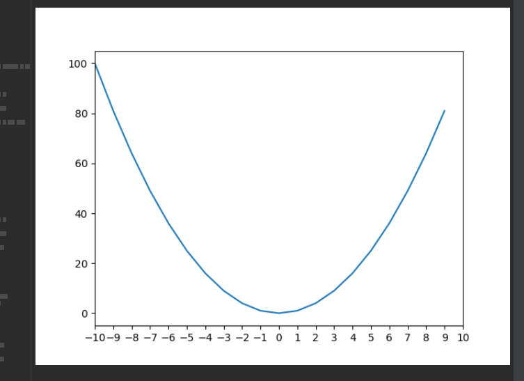
plot:基本画图
import numpy as np\
import matplotlib.pyplot as plt\
\
# We plot the graph of y = x\^2\
x = np.arange(-10, 10) # x coordinate 默认生成-10到10,步长为1\
y = x**2 # y coordinate
[# 明确指定x轴范围,从-10到10 它会把图像的 x 轴范围限制从 -10 到
10。图上超出这个范围的内容会被裁剪掉,不显示。]{.mark}
[plt.xlim(-10, 10)]{.mark}
[# 这是 设置 x
轴的刻度位置(ticks),也就是图上横轴上显示的数字标签。]{.mark}
[np.arange(-10, 11, 1) 生成从 -10 到 10 的整数列表(含 10),步长为
1。]{.mark}[所以会在 x 轴上显示这些刻度(tick marks),比如 -10, -9, ..., 0,
..., 9, 10。]{.mark}[它不会改变x轴的范围,只是控制标签显示的位置。]{.mark}
[plt.xticks(np.arange(-10, 11, 1))]{.mark}
# 以上这两句话虽然有一些overlap,但是通常综合一起使用确保刻度可控
plt.plot(x, y) # Plot the graph\
plt.show() # You need to call plt.show() to show the plotted graph
该代码作图如下:
 {width=”3.178889982502187in”
height=”2.309346019247594in”}
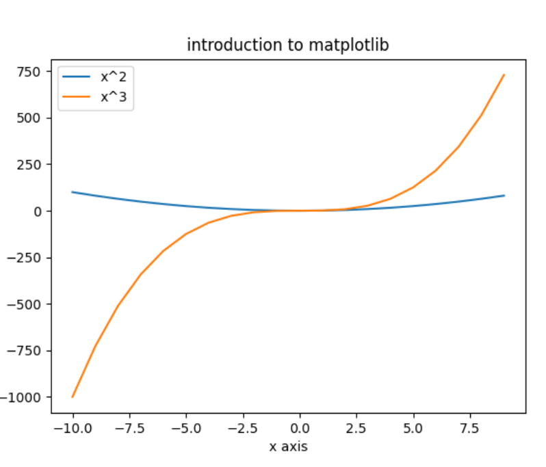
Multiple Functions
#-------------------- Multiple Functions\
\
import numpy as np\
import matplotlib.pyplot as plt\
\
# Create the x and y coordinates\
x = np.arange(-10, 10)\
y1 = x**2\
y2 = x**3\
\
# Plot multiple functions\
plt.plot(x, y1)\
plt.plot(x, y2)\
plt.xlabel(\’x axis\’)\
plt.ylabel(\’y axis\’)\
plt.title(\’introduction to matplotlib\’)
# legend可以放多个函数\
plt.[legend]{.mark}([\’x\^2\’, \’x\^3\’])\
plt.show()
 {width=”2.531898512685914in”
height=”2.16701990376203in”}
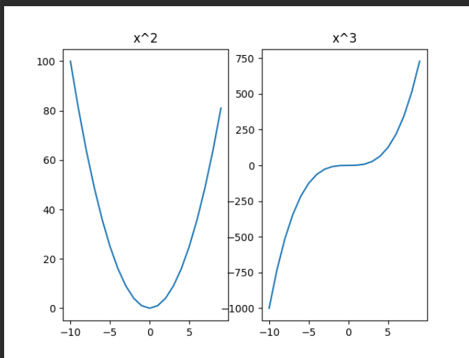
SubPlot:子图
Plot通常指折线图、图表等,figure指整个图片布局
Sometimes we want to can plot different funtions in the different plot
but in the same figure, in this case we can use the subplot function.
 {width=”2.8715627734033244in”
height=”2.192911198600175in”}
import numpy as np\
import matplotlib.pyplot as plt\
\
# subplot(nrows, ncols, plot_number)\
# Arugments are number of rows and colums of the plot\
# and the active plot number\
\
# Create the x and y coordinates\
x = np.arange(-10, 10)\
y1 = x**2\
y2 = x**3\
\
# Create a subplot grid with 1 row and 2 colums\
# and set the active plot number to 1\
# 看你画图,此处布局必须对否则会报错。这个从1计起。\
# 1行,3列,第三个参数是
你正在要画第几个表。第三个参数必须小于等于第二个参数。\
plt.subplot(1, 3, 1)\
\
# Make the first plot at the active plot\
plt.plot(x, y1)\
plt.title(\’x\^2\’)\
\
# Set the active plot number and make the second plot\
plt.subplot(1, 3, 2)\
plt.plot(x, y2)\
plt.title(\’x\^3\’)\
\
plt.subplot(1, 3, 3)\
plt.plot(x, y2)\
plt.title(\’x\^3\’)\
\
# Show the figure.\
plt.show()
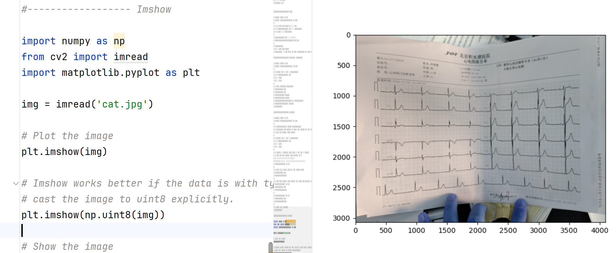
Imshow
import numpy as np\
from cv2 import imread\
import matplotlib.pyplot as plt\
\
img = imread(\’cat.jpg\’)\
\
# Plot the image\
plt.imshow(img)\
\
# Imshow works better if the data is with type unit8, here we\
# cast the image to uint8 explicitly.\
plt.imshow(np.uint8(img))\
\
# Show the image\
plt.show()
 {width=”4.227080052493438in”
height=”1.740501968503937in”}
PyTorch Tensors
Tensor Initialization
# Tensors can be created directly from data. The data type is
automatically inferred.\
\
import torch\
import numpy as np\
data = [[1,2], [3,4]]\
x_data = torch.tensor(data)\
print(x_data)\
\
# Tensors can be created from Numpy arrays (and vice versa)\
\
import numpy as np\
np_array = np.array(data)\
print(np_array)\
x_data = torch.from_numpy(np_array)\
print(x_data)\
\
# We can also call torch.tensor() with the optional dtype parameter,
which will set the data type. Some useful datatypes are: torch.bool,
torch.float, and torch.long\
\
import torch\
data = [[1,2], [3,4]]\
x_data = torch.tensor(data, dtype=torch.float)\
print(x_data)\
\
import torch\
data = [[1,2], [3,4]]\
x_data = torch.tensor(data, dtype=torch.bool)\
print(x_data)
检查数据类型
import torch
x = torch.rand(3,2)
print(x.dtype)
检查shape
import torch
x = torch.Tensor([[11, 12], [13, 14], [15, 16]])
print(x.shape)
输出:
torch.Size([3, 2])
或者直接检查某维度:
import torch\
x = torch.Tensor([[11, 12], [13, 14], [15, 16]])\
print(x.shape)\
print(x.size(0))
形状变动
import torch\
x = torch.Tensor([[11, 12], [13, 14], [15, 16]])\
print(x.shape)\
\
# we can change the shape from (3,2) to (2,3)\
x_view = [x.view(2,3)]{.mark}\
print(x_view)\
\
# You can also use torch.reshape() for this\
x_reshaped = [torch.reshape(x, (2,3))]{.mark}\
print(x_reshaped)
Tensor from a Numpy Array
[注意]{.mark}:NumPy 的默认数据类型(dtype)不一定等于 PyTorch Tensor
的默认 dtype。
# 当 dtype 不是默认的 torch.float32 或 torch.int64
时,会特别显示出来,方便你辨识。\
# 如果 dtype 是默认的(如 int64, float32),打印时不会特别显示
dtype,否则会显示\
\
import numpy as np\
import torch\
data = [[1,2], [3,4]]\
ndarray = np.array(data)\
# 如果要特别指定 dt (数据类型)\
# [x_tensor = torch.from_numpy(ndarray).to(torch.int64)]{.mark}\
x_tensor = torch.from_numpy(ndarray)\
print(x_tensor)
From existing Tensor
你看到的这些数字后面的 [.(小数点)]{.mark} 是因为:
你在代码中写的是浮点数(如 4.),所以 PyTorch 默认创建的是 float32 或
float64 类型的
\
initial_tensor = torch.tensor([[4., 5.], [6., 7.]])\
print(initial_tensor)
[tensor([[4., 5.],]{.mark}
[[6., 7.]])]{.mark}
initial_tensor = torch.tensor([[4, 5], [6, 7]])\
print(initial_tensor)
[tensor([[4, 5],]{.mark}
[[6, 7]])]{.mark}
Code
import torch\
\
# 你看到的这些数字后面的 .(小数点) 是因为:
你在代码中写的是浮点数(如 4.),所以 PyTorch 默认创建的是 float32 或
float64 类型的\
initial_tensor = torch.tensor([[4., 5.], [6., 7.]])\
print(initial_tensor)\
\
# initial_tensor = torch.tensor([[4, 5], [6, 7]])\
# print(initial_tensor)\
\
# Initialise a new tensor of 1s\
# 创建一个和 initial_tensor 形状一样、dtype 一样的全 1 的新 tensor。\
# 这个 1s 是说 ones,就是每个元素都是 1\
new_tensor_ones = torch.ones_like(initial_tensor)\
print(new_tensor_ones)\
\
# Initialise a new tensor of 0s\
new_tensor_zeros = torch.zeros_like(initial_tensor)\
print(new_tensor_zeros)\
\
# tensor elements sampled from uniform distribution between 0 and 1\
new_tensor_rand = torch.rand_like(initial_tensor)\
print(new_tensor_rand)\
\
# tensor elements sampled from a standard normal distribution\
new_tensor_randn = torch.randn_like(initial_tensor)\
print(new_tensor_randn)
输出:
tensor([[4., 5.],
[6., 7.]])
tensor([[1., 1.],
[1., 1.]])
tensor([[0., 0.],
[0., 0.]])
tensor([[0.7206, 0.8806],
[0.9344, 0.1921]])
tensor([[ 0.0496, 1.0113],
[-1.1891, -1.1005]])
Torch随机数rand和randn
想生成**[0,1)** 范围的随机数 → 用 rand_like
想生成有正有负、符合正态分布的噪声或权重初始值 → 用 randn_like
✅ torch.rand_like() vs torch.randn_like()
函数名 取值范围/分布 常用场景
torch.rand_like(t) [0.0, 1.0) 随机初始化(非负)
均匀分布(uniform)
torch.randn_like(t) 正态分布 N(0, 1),均值 权重初始化、模拟噪声
0,标准差 1
形状-->实例化🡪张量
根据shape初始化
There are many ready methods where we can instantiate tensors by
specifying their shapes,
namely, torch.zeros(), torch.ones(), torch.rand(),
and torch.randn()
比如 shape=(2, 3, 4) 生成的数字个数就是 2*3*4 = 24
import torch
shape = (2, 3, 4)
x_zeros = torch.zeros(shape)
print(x_zeros)
x_ones = torch.ones(shape)
print(x_ones)
torch.manual_seed(142)
random = torch.rand(shape)
print(random)
直接arange生成一维数组
import torch\
x = torch.arange(start=0, end=10, step=2)\
print(x)
We can also check the size of a particular dimension of a tensor
using size() method.
import torch
x = torch.Tensor([[11, 12], [13, 14], [15, 16]])
print(x.shape)
print(x.size(0))
指定设备存储张量(为何tensor必须指定设备)
CPU 内存 和 GPU 内存 是两个物理上不同的区域。
一个张量只能在某一块内存中存在,要用 GPU
算法计算,就必须先把数据放进 GPU。
举个比喻:
就像你有两个工作台(CPU 和 GPU),你不可能在 CPU 的桌子上用 GPU
的工具干活,工具(函数)和材料(数据)得在一个地方。
高效计算需要明确位置
- 如果张量位置不一致(比如一个在 CPU、另一个在
GPU),就没法直接进行操作,会抛错。
a = torch.tensor([1, 2]).to(\’cuda\’)
b = torch.tensor([3, 4]) # 默认在 CPU
a + b # ❌ 会报错:Expected all tensors to be on the same device
import torch\
x = torch.Tensor([[7, 8], [9, 10], [15, 17]])\
print(x)\
\
# Determine on which device tensor is stored\
print(x.device)\
\
# Check if a GPU is available; if so, move the tensor to the GPU\
print(torch.cuda.is_available())\
\
if torch.cuda.is_available():\
# [x.to(\’cuda\’)]{.mark} #
这是[无意义操作]{.mark},**.to(\’cuda\’) 并不会修改原始的张量
x,它只是返回了一个新张量,这个新张量才在 CUDA 上。\
# 而你没有接住这个新张量,就相当于: # 新张量被创建 # 你没保存它 #
它立即被销毁 # x 仍然在 CPU 上\
[# 正确写法:\
x = x.to(\’cuda\’)**]{.mark}\
print(\”To cuda successfully\”)\
print(x.device)
tensor操作
加减乘除
跟Numpy差不多
import torch\
x = torch.tensor([1, 2, 3], dtype=torch.float)\
y = torch.tensor([4, 5, 6], dtype=torch.float)\
print([x+y]{.mark})\
\
# you can also use torch.add()\
print([torch.add(x,y)]{.mark})
import torch\
x = torch.tensor([1, 2, 3], dtype=torch.float)\
y = torch.tensor([4, 5, 6], dtype=torch.float)\
\
print(torch.add(x,y))\
print(torch.add(x,y).[sum]{.mark}())
输出:tensor([21]{.mark}.) 因为全部的数加在一起就是21
Dot Product and Matrix Multiplication
点乘
import torch
x = torch.tensor([1, 2, 3], dtype=torch.float)
y = torch.tensor([4, 5, 6], dtype=torch.float)
# Dot product
print(x.[dot]{.mark}(y))
矩阵乘
import torch\
x = torch.tensor([[1, 2, 3], [4, 5, 6]], dtype=torch.float)\
y = torch.tensor([[1, 2], [3, 4], [5, 6]], dtype=torch.float)
三种矩阵乘法的表示
# Matrix Multiplication\
print(torch.matmul(x, y))\
\
# you can also use torch.mm()\
print(torch.mm(x, y))\
\
# or you can use x@y\
print(x@y)
合并
import torch\
\
# creating a tensor\
x = torch.ones(2, 2, 4)\
print(x)\
\
y = torch.ones(2, 2, 4)\
print(y)
# cat是粘贴的意思,dim是说沿着第几维度进行合并
z_cat = torch.cat([x, y], [dim]{.mark}=2)
# z_cat = torch.cat([x, y], dim=1)\
print(z_cat)
Google colab
就是Google云端Jupyter,可以指定runtime的显卡来运行一些tensor
 {width=”5.768055555555556in”
height=”2.295138888888889in”}
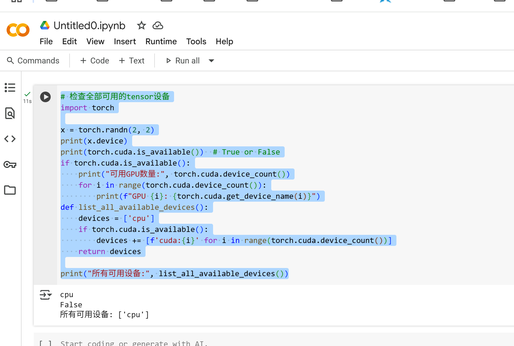
代码:python检查当前tensor的全部可用设备
# 检查全部可用的tensor设备
import torch
x = torch.randn(2, 2)
print(x.device)
print(torch.cuda.is_available()) # True or False
if torch.cuda.is_available():
print(\"可用GPU数量:\", torch.cuda.device_count())

for i in range(torch.cuda.device_count()):

    print(f\"GPU {i}: {torch.cuda.get_device_name(i)}\")
def list_all_available_devices():
devices = \[\'cpu\'\]

if torch.cuda.is_available():

    devices += \[f\'cuda:{i}\' for i in
range(torch.cuda.device_count())]
return devices
print(\”所有可用设备:\”, list_all_available_devices())
设置仅cpu
 {width=”5.768055555555556in”
height=”3.8833333333333333in”}
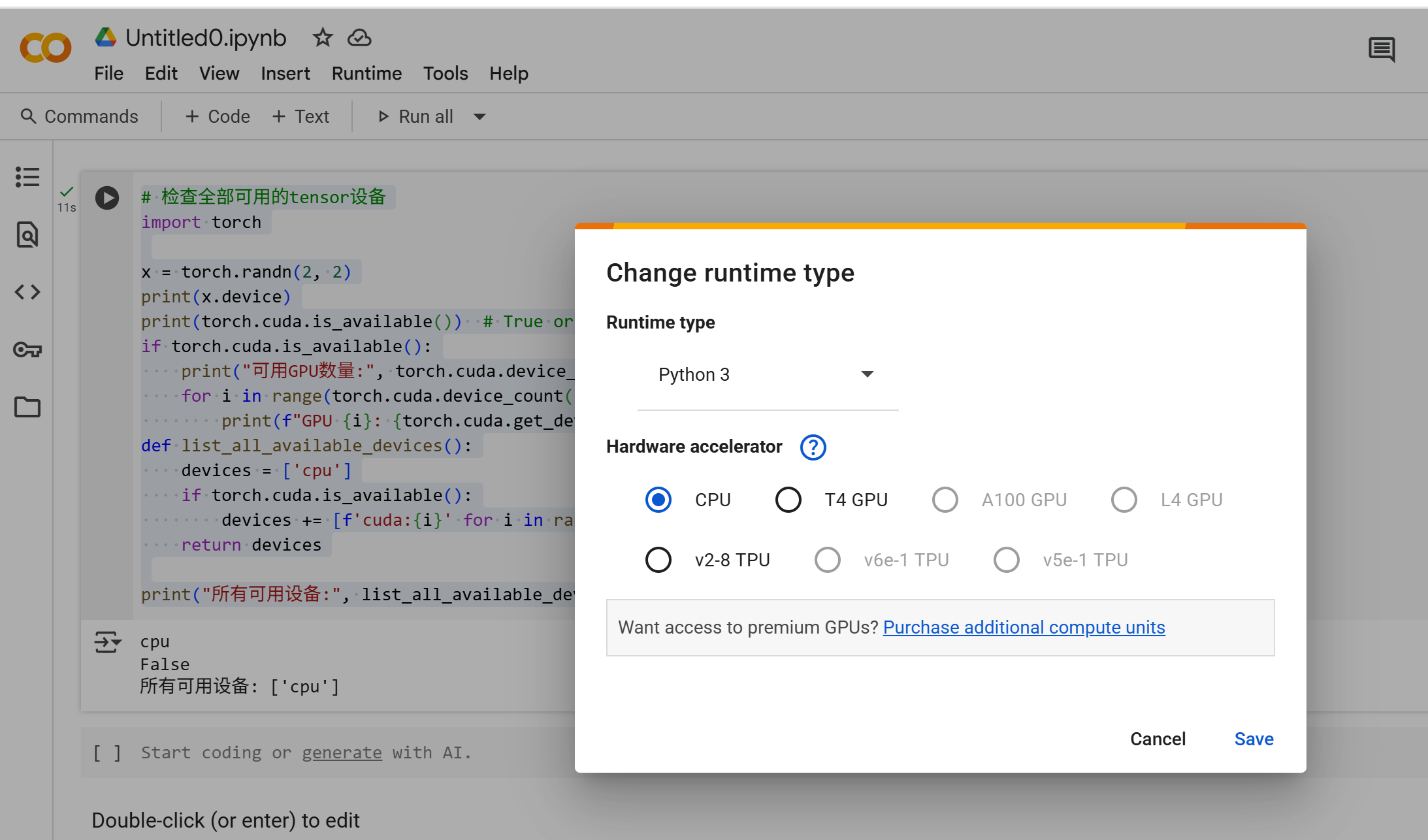
设置TPU的runtime
Runtime -> change runtime type -> 改TPU
 {width=”4.124489282589677in”
height=”2.426228127734033in”}
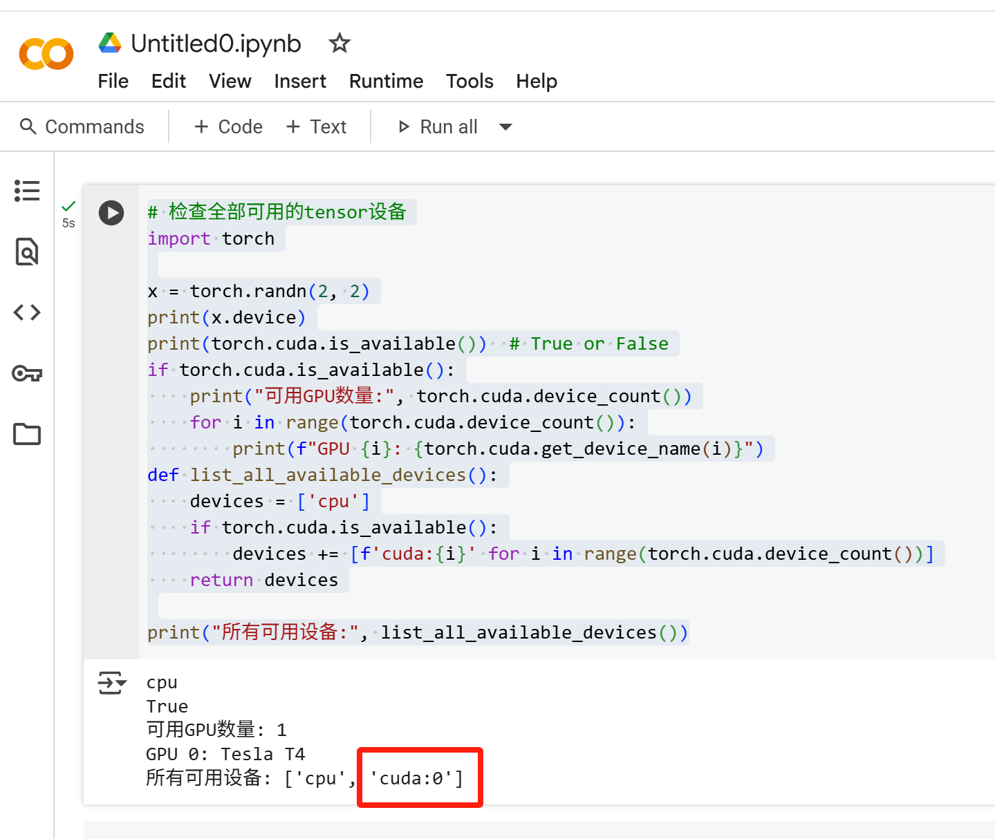
我改T4 TPU
 {width=”4.136831802274716in”
height=”3.4898600174978127in”}
发现Tesla T4 显卡
Welcome to point out the mistakes and faults!